Tapered Bezier curve for Fusion

I want a better Lightning tool for Fusion. The existing one, a fuse that was available in VFXPedia prior to the Blackmagic takeover, was never really good enough for production. As a result, any time I’ve wanted electricity effects, I’ve fallen back on After Effects. I’ve had some ideas about how to improve the Lightning Fuse, but when it came time to actually open it up and make some changes, I ran into two problems: Fusion can’t draw a tapered spline, and the BezierTo() method for the Fuse drawing API is broken. Solving one of those problems offered me the opportunity to solve both at once, so that’s what I did.

In this developer’s diary, I’ll walk through the creation of a tapered Bezier curve Fuse. All of my testing was done in Fusion 9. I have no reason to expect that the fuse won’t work in v16 or Resolve, but I haven’t tried it yet. I hope that I’ll be able to extend what I’ve done here into that Lightning Fuse, but that’s a few steps down the road. I’ll be certain to document it when I get there.

Step 1 was to figure out exactly how a Bezier curve is drawn in the first place. There are quite a few places to look, but one of the most entertaining (to me) was the Pixar in a Box videos at Khan Academy. That introduced me to De Casteljau’s algorithm, which is what I ultimately used to create the curve. I’ll get to that big polynomial and its application a little later. For now, take some time to watch the Pixar videos and get an intuitive understanding of the process we’ll use.

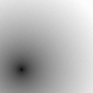
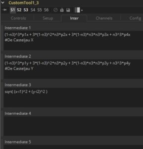
Step 2 was learning how to actually draw something with Fusion. If you happened to glance at some of those OpenCL experiments I did a while back, you’ll already be familiar with the approach I tried first: Test each pixel to see how far it is from the curve, and use that distance field to determine what color the pixel should have. I set up a few CustomTools with various expressions, building a little library of solutions for drawing shapes. Then it came time to solve De Casteljau, which is a gigantic mess of a polynomial:

(1-t)³ * p1 + 3 * (1-t)² * t * p2 + 3 * (1-t) * t² * p3 + t³ * p4 = P

p1 – p4 are the four control points for the curve, and the resultant, P, is the coordinate of a point on that curve. t represents displacement along the curve—a position somewhere between p1 (t = 0) and p4 (t = 1). I plugged that into a CustomTool, used one of the Number In sliders for t, and found the distance of each pixel from P. That let me slide a disc along the described curve, but it wouldn’t allow me to actually draw the curve.

I’d run into a similar issue drawing a simple line, so I went back to that to remember what I’d done. I had the parametric equation of a line: P = p1 + p2 * t. Solving that one involved breaking it out into vectors and finding a way to set the two vectors equal to one another:

X = x1 + x2 * t
Y = y1 + y2 * t

t = (X – x1) / x2 = (Y – y1) / y2

Therefore:

X = x1 – ((y1 – y) * (x1 – x2)) / (y1 – y2)
Y = y1 – ((x1 – x) * (y1 – y2)) / (x1 – x2)

Following that same logic, I figured I could break the equation into vectors, solve for t, and then set the two vectors equal to one another. Now look back at that polynomial up there.

Solve for t… Right. Not happening.

Nevertheless, the Custom Tool experiment did verify that the math worked, and if I could find a way to use it, then I’d have something usable. My ultimate goal was to build a Bezier method for Fuses, so I abandoned Custom Tool in favor of getting in and writing some actual code.

I’ve described the basics of Fuse writing before, so I won’t go into much depth about that. Let’s start straightaway with the Bezier solver:

function solvePoint(p1, p2, p3, p4, t)
	local p = {}
	p.X = (1-t)^3*p1.X + 3*(1-t)^2*t*p2.X + 3*(1-t)*t^2*p3.X + t^3*p4.X
	p.Y = (1-t)^3*p1.Y + 3*(1-t)^2*t*p2.Y + 3*(1-t)*t^2*p3.Y + t^3*p4.Y

	return p
end

The function takes the four control points and the t value and returns a single point on the curve. I can think of two ways to use this information. First, I could use my previous approach, as seen in the Voronoi or OpenCL Fuses I’ve written before, and try to find the distance between each pixel and the nearest point on the curve. Although it’s how I’ve done things before, it’s not a trivial problem in this case. It’s not how I wrote this Fuse, but I think I’d like to talk through it anyway.

This is a good candidate for a ‘divide-and-conquer’ approach. The idea being to do the smallest possible number of solves in order to get to the result. First, for any given pixel, I’d check to see if it is inside the bounding box formed by the four control points—the Bezier curve will always exist entirely inside that box, and solving that problem is faster than running solvePoint(). Assuming the pixel is still a candidate, I’d compare it to a pre-computed list of t-value/point pairs, looking for the two closest. That would be similar to the process performed in the Voronoi fuse. Then there would probably be some variant on a binary search along the curve between those two points looking for a minima (within a pre-determined level of uncertainty—half a pixel, perhaps). Finally, I’d calculate the distance between the pixel and that point. I may one day code that solution, but it’s a bit more involved than what I actually did, and it would require me to do some work on rendering, which I get to skip in the approach I actually took.

The second possibility is the one I actually implemented, and that was to subdivide the curve and approximate it using very short line segments and Fusion’s existing Drawing API. To start, I need a Shape and a variable to hold it, as well as the t variable and another variable to hold the results of solvePoint():

local line1 = Shape()
local t
local s = {}

Since at t = 0, P = P1, I can just start there:

line1:MoveTo(P1.X, convertY(P1.Y, img))

The function convertY() takes a Y coordinate and corrects for a non-square image aspect:

function convertY(y, ref_img)
	return y * (ref_img.Height * ref_img.YScale) / (ref_img.Width * ref_img.XScale)
end

Once the start point has been determined, it’s simple to loop through any number of t values, building the curve from small line segments, the number of which is determined by the subdivs variable, exposed on the control panel as “Smoothness”:

for i=0,subdivs do
	t = i/subdivs
	s = solvePoint(P1,P2,P3,P4, t)
	line1:LineTo(s.X, convertY(s.Y, img))
end

And then style the line:

local outlinetypes = {"OLT_Solid", "OLT_Dash", "OLT_Dot", "OLT_DashDot", "OLT_DashDotDot",}
line1 = line1:OutlineOfShape(thickness, outlinetypes[linetype], "OJT_Round", (req:IsQuick() and 8 or 16))

The variables linetype and thickness are taken from control panel inputs. “OJT_Round” is the cap shape on the end of the line. The last argument determines the anti-aliasing quality of the line: 8 if the HiQ switch is off, and 16 if it’s on.

So that’s the basics on drawing the curve. But what about tapering it? Assuming the user wants some control over the length of the taper, that requires adding some more controls. I really wanted to use a SplineControl, which would open up other possibilities for shaping the spline in addition to just tapering it, but accessing the contents of a LookUpTable is apparently something you need Fusion 16 for, and I’m not ready to migrate there yet. So this Fuse will just use a pair of Range controls—one for each end of the curve, which are easier to animate, anyway.

Outside the loop, the only thing that changes is the nature of the line variable. Trying to apply a different thickness to each line segment of a single shape turned out to be extremely slow, so this time the line will be a table that holds many Shape objects instead of being a single Shape.

Inside the loop, I use an intermediate variable called modthickness to hold the modified value of thickness that will be applied to each segment. There are two cases for tapering: We’re measuring either from the start of the curve (P1) or the end (P4). It’s simple enough to just divide the curve in half at t = 0 and treat them separately.

local s = {}
local r = {}
local line = {}

for i = 1, subdivs do
	local modthickness = 1
	local t = i/subdivs
	local t2 = (i-1)/subdivs --Fix for the taper hitting 0 prior to reaching P4

	if t < 0.5 then
		modthickness = thickness * math.min(t/endTaper1, 1)
	else
		modthickness = thickness * math.min((1-ts)/(1-startTaper2), 1)
	end

	if t < startTaper1 or t2 > endTaper2 then modthickness = 0 end

	line[i] = Shape()
	s = solvePoint(P1,P2,P3,P4, (i-1)/subdivs)
	line[i]:MoveTo(s.X, convertY(s.Y, img))
	r = solvePoint(P1,P2,P3,P4, t)
	line[i]:LineTo(r.X, convertY(r.Y, img))
	line[i] = line[i]:OutlineOfShape(modthickness, outlinetypes[1], "OJT_Round", (req:IsQuick() and 8 or 16))
end

Each line segment is a separate shape and can therefore have its own thickness, so the OutlineOfShape call was moved inside the loop. The min() statements ensure that once t exceeds the appropriate taper threshold the thickness does not keep increasing. In the case of t > 0.5, I have inverted the values in order to measure from the end. I found that the curve tapered out early when doing that, so t2 adds an extra “ghost” segment beyond t = 1 to compensate.

Unfortunately, from the perspective of the drawing API, each segment of the curve exists all on its own, so the outline types no longer work. I’ve locked that argument to the Solid style. In addition, the Smoothness needs to be turned up much higher for the tapering curve in order to disguise the stair-step patterns near the end points. The shorter the taper, the higher the Smoothness has to be to compensate.

My next task is to figure out if I can manage to replace the existing BezierTo() method in the drawing API with my new and improved version so that work on the Lightning Fuse can move forward. I’m also rather eager to see what can be done by the likes of Dunn Lewis, creator of the excellent FUI series of fuses, available in Reactor.

Here’s the complete Fuse:

MT_BezierTapered.fuse