This is the sixth in a series of articles in which I explore the lessons recommended by Vivo & Lowe's Book of Shaders in the context of custom Fuse tools for Blackmagic Fusion.
In the previous article, I learned how to use OpenCL to create some basic shapes, and during that process I set up some Translate and Scale controls so that I could use the Viewer widgets I'd set up to control the shapes. I mentioned that I suspected my approach to scaling was unorthodox, but as it turns out from reading the BoS's 2D Matrices chapter, I did it exactly right: Rather than moving the shape, I modified the coordinate system, effectively reshaping the world around the shape. In so doing, I actually ran ahead of the lessons a little and solved 2/3 of this chapter already.
Furthermore, I almost used the trigonometry I already knew to perform rotations, but I second-guessed myself and held off on that. As it turns out the matrix multiplication method demonstrated in BoS is just the trigonometry rotation formulae dressed in different clothes. Here are the equations I already know for a 2D rotation:
x' = x * cos ϴ – y * sin ϴ
y' = x * sin ϴ + y * cos ϴ
The rotation matrix operation given at BoS is this:
Well, that looks like the exact same operation to me! I suspect there is more power in the use of matrices than these basic transforms show, but for the level I'm at right now, it seems that using matrix functions is rather unnecessary. Of course, that means I'm putting off learning more about that topic in favor of getting a more immediate result using information I already have. That will bite me later, I'm sure.
Translation
In the previous version of the Fuse, I packed my transformations into the shape drawing kernels. While it's pretty efficient in terms of how many lines of code I use, it makes the resulting kernels a little bit difficult to read and understand. Furthermore, it means that I have to pack all of that code into each shape function. By breaking the transformations out into separate functions, everything becomes less confusing. Let's start with translation:
st -= ctr - 0.5f;
The Center control defaults to a location of 0.5, which is also the center of the canvas. In order to place the widget in the center of the screen but still have it act as though that location were the origin, I need to subtract 0.5 from it in order to "zero out" its own default value. Since I'm sliding the coordinate system around instead of the actual shape, I also subtract rather than adding. As the world slides left, the shape appears to slide right.
In the shape functions, I can remove references to ctr and instead simply call a transShape() function:
float2 transShape(float2 st, float2 ctr)
{
return st -= ctr-0.5f;
}
Scale
The scaleShape() function is a little more complex because I want to be sure that I am scaling from the correct pivot, which is the location of the Center control:
float2 scaleShape(float2 st, float2 scale, float2 ctr)
{
//Move center to origin
st -= ctr;
//Multiply
st *= scale;
//Move center back
st += ctr;
return st;
}
I no longer want to create my rectangle at the final size. Instead, I make it fill the entire screen, then stretch or squeeze the coordinate system around it. Just like with translation, though, I need to invert the scale factor in order for it to work correctly. Inverting a translation is as easy as changing addition to subtraction. A scaling operation is multiplication, so to invert it I need to instead divide. Just like with ellipsesz in the last article, though, I'm nervous about taking the reciprocal of a variable, so I add an infinitesimal to it before making the function call:
//Scale
float2 scale = 1.0f/(rectsz+0.000001f);
st = scaleShape(st, scale, ctr);
A New Rectangle Function
With these to functions in hand, I was able to simplify the shape creation code, but I went right ahead and complicated it again by changing from a step() to a smoothstep():
//Create positive
float2 bl = smoothstep(1.0f+iborder+isoftness, 1.0f+iborder-isoftness, st);
float2 tr = smoothstep(1.0f+iborder+isoftness, 1.0f+iborder-isoftness, 1.0f-st);
float pos = bl.x * bl.y * tr.x * tr.y;
Notice that I've added a new variable into the mix (and thus a new parameter for the rectangle() kernel. Softness comes in from a Soft Edge control on the panel. This procedure produces something very similar, if not identical to, Fusion's Multi-Box filter with Num Passes set to 2. I corrected the image aspect ratio of the softness just like the border width correction I performed in the last article. I also discovered that smoothstep() breaks if the edges are identical, so I added another infinitesimal to softness to prevent that condition.
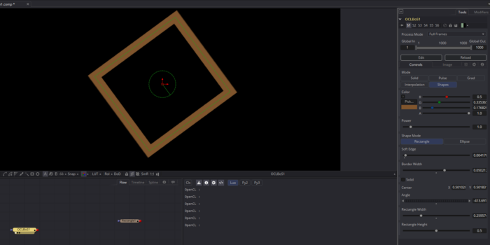
With a functioning rectangle() kernel, I started testing my code. For the most part it worked as I expected, but translation was very strange—there seemed to be some kind of multiplier on the control that made the rectangle move further than its center control. This turned out to be another consequence of manipulating the coordinate system rather than the object. While the usual order of operations for a transformation is Translate, Rotate, Scale, if you are manipulating the world, then the scaling also performs an additional translation. I had to reverse the order to get the expected results, translating at the end of the chain instead of the beginning.
The rectangle() function has changed so much by this time that I'll offer it to you in its entirety:
kernel void rectangle(FuWriteImage_t img, int2 imgsize, float4 col,
float2 rectsz, float2 ctr, float angle, float border,
int solid, float softness)
{
int2 ipos = (int2)(get_global_id(1), get_global_id(0));
float solidf = 1.0f - convert_float(solid);
//normalize the pixel position
float2 iposf = convert_float2(ipos);
float2 imgsizef = convert_float2(imgsize);
float2 st = iposf/imgsizef;
//correct for image aspect ratio float
aspect = imgsizef.x/imgsizef.y;
float2 iborder = (float2)(border, border*aspect);
//Fix softness bug
softness += 0.00001f;
float2 isoftness = (float2)(softness, softness*aspect);
//Scale
float2 scale = 1.0f/(rectsz+0.0000001f);
st = scaleShape(st, scale, ctr);
//Rotate
st = rotShape(st, angle, ctr);
//Translate
st = transShape(st, ctr);
//Create positive
float2 bl = smoothstep(1.0f+iborder+isoftness, 1.0f+iborder-isoftness, st);
float2 tr = smoothstep(1.0f+iborder+isoftness, 1.0f+iborder-isoftness, 1.0f-st);
float pos = bl.x * bl.y * tr.x * tr.y;
//Create negative
float2 bln = smoothstep(1.0f-iborder+softness, 1.0f-iborder-softness, st);
float2 trn = smoothstep(1.0f-iborder+softness, 1.0f-iborder-softness, 1.0f-st);
float neg = bln.x * bln.y * trn.x * trn.y;
//Delete interior, if necessary
float pct = pos * (1.0f - solidf*neg);
//Set color float3 rgb = (float3)(pct * col.xyz);
//Set output
float4 outcol = (float4)(rgb*col.w, pct*col.w);
//Create output buffer
FuWriteImagef(img, ipos, imgsize, outcol);
}
Rotation
I was all set to ignore my previous decision to skip learning about matrices, only to discover that OpenCL apparently doesn't have any matrix data types or handling methods built-in. I would therefore have to build the infrastructure for handling a matrix before I could even use it. So I'll rely on my initial instinct to just use what I know. Fortunately, while researching the issue, I also came across a place where my Fuse-based solution will actually be faster than the BoS code.
The GLSL examples on BoS are executed in parallel on the GPU. Every pixel in the canvas has to do all of the calculations involved in each operation, even if every single pixel would get the same value. I, on the other hand, can perform certain precalculations in the serially-executed Process() function of my Fuse and then pass the results into the kernel as an argument. Specifically, I can calculate sin ϴ and cos ϴ on the CPU just once instead of having to do it tens of thousands of times on the GPU.
angle = angle * math.pi/180 * -1
local sin_theta = math.sin(angle)
local cos_theta = math.cos(angle)
That first line converts degrees to radians. My existing code is already importing an angle argument. I had intended to just feed theta in there, but with a couple of tiny tweaks—changing float angle to float2 angle and prog:SetArg(kernel, 5, angle) to prog:SetArg(kernel, 5, sin_theta, cos_theta)—I can change that into a vector and use it to hold the results of sin and cos instead. Now, angle.x holds sin ϴ and angle.y holds cos ϴ.
From here, things started breaking down for me. I eventually sorted out the order of operations: rotate, scale, then translate. Where exactly to correct for the aspect ratio took a bit longer. That apparently needs to be done in the rotation formulae themselves, so I had to pass aspect into rotShape(). But getting that right disturbed my scaling calculations, so I then had to bring aspect into the scaleShape(), too. And doing that made my aspect correction on the border width invalid, so I removed that.
Rotation is hard.
Eventually, though, I did get everything working as expected.
Generalization
Now I need to make sure that my generalized transformation functions will work just as well for the Ellipse as they do for the rectangle. For the most part it does. I had to put in an anti-correction for the aspect ratio in the call to Scale:
st = scaleShape(st, (float2)(scale.x,scale.y/aspect), ctr, aspect);
And for some reason, the smoothstep() doesn't produce the same amount of blurring on the ellipse as it does on the rectangle. I multiplied softness by 3 to compensate:
//Create shape
float pos = smoothstep(1.0f + softness*3.0f, 1.0f - softness*3.0f, (dot(st-0.5f, st-0.5f)*4.0f)-border);
float neg = 1.0f - smoothstep(1.0f - softness*3.0f, 1.0f + softness*3.0f, (dot(st-0.5f, st-0.5f)*4.0f)+border);
As Chad pointed out in a comment on the previous article, the multiplication by 4 in the dot product method is not actually arbitrary, and it does eliminate the need for sqrt(), so I have used it here, in addition to swapping softstep() for step().
The two shape kernels are now simpler, with transformations moved out into shared functions. This gives me the opportunity to easily add additional shape kernels without having to solve those problems over and over. Of course, I won't have accurate on-screen widgets for anything other than rectangles and ellipses. Skipping back to BoS chapter 7, let's take a look at a regular polygon with an arbitrary number of sides.
Polygon
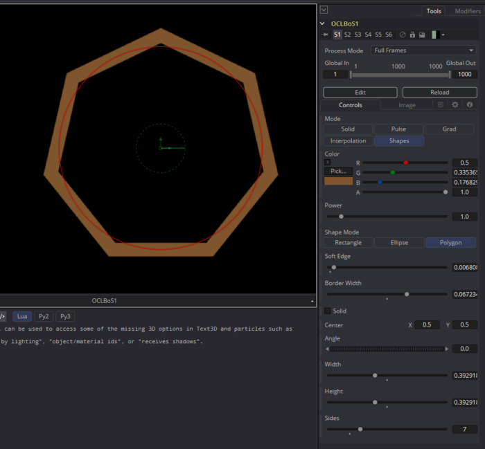
At long last, I'll be creating something that isn't trivial to make with other Fusion nodes! Everything up to this point has been merely variations on existing tools, but making a regular polygon with an arbitrary number of sides is new. This algorithm can be found at the bottom of the BoS' Shapes chapter, under the heading "Combining Powers." I'll try to break down the math as I go, mostly for my own benefit.
My new kernel opens with what is becoming a standard set of instructions for shape creation, now including the three transformation function calls. From there, I remap the coordinate space to operate in a range of -1.0 to +1.0:
st = st * 2.0f - 1.0f;
The technique we'll be looking at uses polar coordinates instead of rectilinear ones, and performing this remap puts (0,0) in the center of the screen, with a four-quadrant environment suitable for angular operations. Next, I find the angle of a ray cast from the center of the screen to the current pixel:
float a = atan2(st.x, st.y) + M_PI;
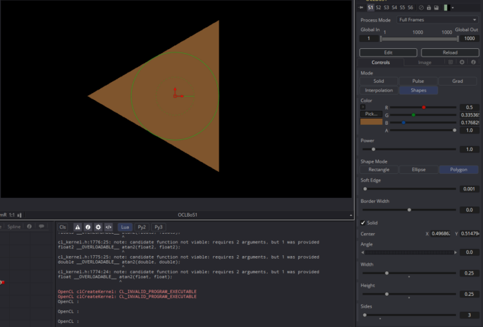
atan2 is the arctangent of y/x. From trigonometry, I know that if a line is at an angle ϴ from the x-axis, the tangent of ϴ is equal to the slope of that line. So the arctangent of that slope yields ϴ. Knowing that, the above expression looks malformed. I've got the slope inverted, and why am I adding π? A little bit of experimentation in my finished kernel reveals to me that these quirks simply rotate the shape to a more intuitive orientation. atan2(st.y,st.x) creates a shape that is anchored on the right edge. Here's the triangle produced by this variation:
Using the reciprocal of the slope, though, trades x for y, reorienting the shape so that it's anchored on the top. Adding π rotates the triangle 180°, putting the anchor on the bottom and giving an upright triangle, which feels more familiar. It also makes some of the upcoming math a little brain-bending since 0° is now straight down. I had to turn my head sideways occasionally to make sense of what was going on.
Next up we have the line that distributes sides around the shape:
float r = M_PI * 2/ sides;
2 * π radians is a full circle (a number sometimes designated tau, or τ). Dividing that circle by the number of desired sides gives the angle through which we'll turn to create each side. Expressed another way, r is the angular length of each side. This notion of angular distances is key to the polar coordinate space.
Next we have a complex formula that distorts the distance field into the desired shape:
float d = cos(floor(0.5f+a/r)*r-a) * length(st);
This guy's a little bit involved. Starting from the deepest part of the nest, we have floor(0.5f + a / r). floor() is a function that rounds a number down. Adding 0.5 to a number to be rounded in this fashion is an easy way to round to the nearest integer. So if we have a ray drawn from the center of the screen through the current pixel, this expression will determine which side of the shape the ray will cross. That integer gets multiplied by r, which gives the angular center of that side. Subtracting a gives the angular distance between the current pixel and the center of the side it "belongs" to. And the cosine of that number gives a factor by which the coordinate system should be scaled along that angle. I think.
The results of cos() should always be less than or equal to 1, and the maxima occur when the angular distance is 0. My intuition tells me that the corners of the shape should be closer to the center than the middle point of each side. As with the transform functions above, though, I realized that stretching the coordinate system has the opposite effect from stretching the shape. I am not making the distance itself smaller, I am changing the definition of the distance, and making that smaller causes the actual screen distance to get larger. I can already tell that this inversion is going to mess with my intuition. Hopefully I'll eventually get used to it.
Here is the newest Fuse: BoS_LessonEight.fuse
The next Book of Shaders chapter is about pattern generation. It starts getting into the meat of why I wanted to learn OpenCL. And of course, I'll continue to refine my understanding of distance fields and shaping functions as I go.


