 A lens flare is an artifact caused by reflections of a bright light source inside the complex lens assembly of a camera. There are thousands of permutations of lens flare appearance, but they can be broken down into a few component elements that are possible to parameterize.
Most of the lens flare tools I've used so far involved tracking a light source and using that data to determine the origin point of the flare. All of the flare's properties are fully controlled by the artist, and occlusion has to be managed with roto mattes or a key.
Some 3d renderers, like Redshift, have a post-fx filter to create lens flares. These depend only on the intensity of rendered pixels and a few parameters, so the motion, occlusion, and evolution of the flare is achieved automatically.
In this exploration, I'd like to look at both approaches on my way to creating one or more lens flare tools for Houdini's new image processing system, Copernicus (COPs). I'll look into existing CG lens flare implementations and also real photographed flares and attempt to reproduce them in the OpenCL COP. First up is a public domain OpenGL flare posted at ShaderToy by mu6k:
https://www.shadertoy.com/view/4sX3Rs
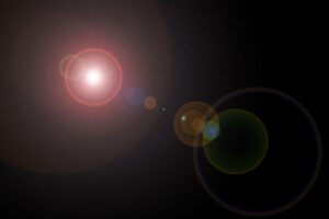
This is an example of the kind of flare I've used in the past. It generates the light source, some god-rays, a couple of "orbs" and a partial halo. The source is quite dramatic and probably not suitable for the kind of application I have in mind, but the reflections are subtler and might be useful. At the very least, it gives me a place to start with my own. At only 120 lines of OpenGL, this should be relatively easy to reproduce.
Setting Up the Frame Buffer
When analyzing code, it's tempting to just start at the top and try to understand everything in the order presented. That's not often the easiest way to do it, as most programs declare a lot of constants and functions at the top that don't make any sense until you've looked at the place where execution begins. So let's start with the mainImage() function. I'll go slowly and carefully because it's very easy to get the OpenCL COP to crash. It's probably also a good idea to keep Houdini's Cache Manager open in order to purge the COP OpenCL Buffer Cache occasionally to prevent VRAM overflows. For the sake of clarity, I'm going to refer to the OpenGL ShaderToy code as ShaderToy and Houdini's OpenCL code as OpenCL. That's less likely to cause confusion due to the similarity in the shading language names.
We get some advantages from the OpenCL COP: We don't need to calculate the normalized uv coordinates or correct for image aspect. All of that is handled by the built-in binding @P. So lines 106 & 107 of the ShaderToy are completely unnecessary.
The next bit of the ShaderToy sets up an odd variable: mouse. This is the location of the user's mouse in the ShaderToy window, and the z component indicates whether or not a button is being clicked. If a mouse button is not being clicked, then the location of the flare comes from some sin waves and the time. When a button is held down, the flare moves to the mouse location. In the version of the tool where the light source location is set with a parameter, I'll make a float2 parameter flaresrc to replace mouse, and I'll replace iMouse.z with a parameter called animate, which will have a simple toggle in the UI.
There's also some strangeness with the sin() functions in the animated version of the ShaderToy, so I'm going to simply use cos() for the x axis and multiply each by 0.5 to get a nice circle going when it's animated. I can add a little chaos by tweaking @Time later, if I feel like it, but it seems likely that I'll eventually dump the animated mode in favor of animating the flaresrc parameter itself.
The next segment of ShaderToy code includes calls to some functions that haven't been set up yet: lensflare(), noise(), and cc(). I'm not going to tackle those immediately, but I still want to test my existing code, so I'll render the image coordinates and a distance field for now.
OpenCL conveniently has a distance() function that does exactly what you'd expect: it returns the distance between two position vectors. I want a bright spot as my flare source, though, so I'll invert the results, giving a radial gradient centered at flaresrc. And for good measure, I'll add a radius parameter so I can control the size of the gradient.
It took some experimentation and a long, slow walk around the office to work out how to get the radial gradient to work the way I wanted. I knew that my radius control was supposed to scale the gradient, which means multiplication, but figuring out when to multiply fooled me for a bit. Since I knew I wanted a bright spot rather than a hole, I'd inverted dist. But when I multiplied that by radius, all I did was adjust the brightness of the spot instead of its size. Instead of multiplying the bright spot, I needed to divide the distance field by radius before inverting it. That way, the gradient shrinks as the radius control is increased, and when inverted it behaves like I want it to. But dividing by a variable is always dangerous, so I first clamped the low end to a very small value, ensuring I'd never divide by 0.
#bind layer src? val=0
#bind layer !&dst
#bind layer noise? val=0
#bind parm flaresrc float2
#bind parm animate int val=0
#bind parm radius float val = 0.01

@KERNEL
{
    float2 flaresrc = @flaresrc;

    if(@animate > 0)
    {
        flaresrc.x = cos(@Time)*0.5;
        flaresrc.y = sin(@Time)*0.5;
    }

    float radius = max(0.001f, @radius);

    float dist = 1.f-(distance(@P, flaresrc))/radius;

    float4 color = (float4)(@P.x, @P.y, dist, 1.0f);

    @dst.set(color);
}
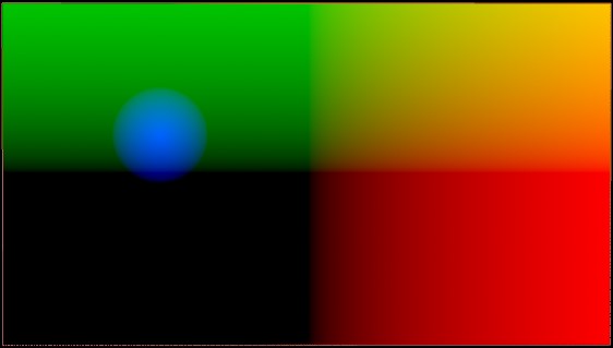
This appears to be working as expected. I have a horizontal gradient in the red channel that visualizes imgcoords.x, a vertical gradient in green to visualize imgcoords.y, and a radial gradient in blue visualizing flaresrc. Of course, it is in image coordinate space, so there are negative pixel values across much of the image, but inspecting the values in the Composite Viewer shows that they're what I expect.
The lensflare() Function
On line 116, the hotspot's color is multiplied by the output of a function called lensflare(), which takes two vectors as input: uv and mouse.xy. As discussed above, we can use @P for uv, and mouse.xy has been replaced with flaresrc. The function is declared on line 52 of the ShaderToy.
This is a pretty long bit of code with quite a few cryptic variables. To best make sense of something like this, I like to look first at its output, which is a vec3 variable called c, declared on line 89. I presume that's meant to be an RGB color. Each channel gets the sum of several of those variables, the whole thing is given a 30% gain up, and then what looks like the distance from the center of the screen is subtracted. The variable uvd looks like it's doing a lot of work here, so I think my next step should be to confirm my intuition about what it is.
The nice thing about a function is that it doesn't care about the variable names in your main program—it will change them to its own input names, so I'll go ahead and match the function declaration from the ShaderToy, even though the variables I'm feeding into it have been renamed. I'll go ahead and set c to black and call for the function just like the ShaderToy does. As expected, my image turns completely black because I am now multiplying RGB by 0.0f. My new color is:
float4 color = (float4)((float3)(@P.x, @P.y, dist)*lensflare(@P, flaresrc), 1.0f);
And the initial lensflare() function is:
float3 lensflare(float2 uv, float2 pos)
{
    float3 c = (float3)(0.0f);
    return c;
}
It will be easier to inspect the results of my code if I remove the gradients I'd set up before. In case I want to come back to them, though, I'll make a copy of the line, modify it, and comment out the original. That way I can easily see what c is doing in isolation:
    //float4 color = (float4)((float3)(@P.x, @P.y, dist)*lensflare(@P, flaresrc), 1.0f);
    float4 color = (float4)((float3)lensflare(@P, flaresrc), 1.0f);
I can test to be sure this works by changing the value of c. As expected, the output color changes, so I know all is well. Now I can start testing uvd. It's a vec2 in ShaderToy, so I'll need to cast float2 to float3 in order to store it in c.
    float2 uvd = uv*(length(uv));
    float3 c = (float3)length(uvd, 0.0f);
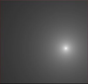
If I put this output directly into the final color, I get a radial gradient around the center. Given that this is subtracted from c, I suspect that it's intended to serve as a vignette, but it would be better to invert it and multiply it by c so as to avoid the possibility of negative pixels. But after multiplying by 0.05, as is done in ShaderToy's line 92, it's effect is negligible. I'll replace that constant with another parameter to make it more pronounced.
The very last thing that happens before we return to the main kernel is the variable f0 is added to c. That one appears to be fairly straightforward, and I suspect it's going to turn out to be the hotspot itself. Let's give it a try and see.
    float f0 = 1.0f/(length(uv-pos)*16.0f+1.0f);
    float3 c = (float3)(0.0f);
    c += (float3)f0;
It's not quite what I'd expected. Looking at the next line, I see that it gets modified by a noise() function, so I'll bet this turns out to be the god rays. To verify that, I'll need to start up yet another new function, and it looks like I'll need to provide a noise field as a second input.
I ran into trouble at this point because the OpenCL COP doesn't permit the bound inputs to be called from functions, and when you pass the bound layer, all you're actually sending is the sampled value at the current fragment. The simplest, and probably best, solution would be to dismantle lensflare() and put it inside the kernel. And when I asked the developers for advice, that's what they told me. But one of them did suggest looking at the generated code to see if I could get some hints, and being stubborn about my process, that's what I did.
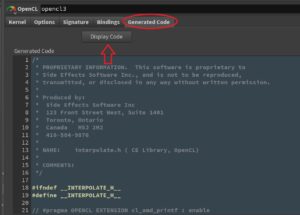 To see aaallll the OpenCL code, switch over to the Generated Code tab and click the Display Code button. For convenience, it's a good idea to open this code in a separate window. You can do that with the Alt+E hotkey. Or you could copy it all into the programmer's text editor of your choice. I prefer Sublime. It might take some long study of what's going on inside here, but you can often get some hints from the error messages the COP provides, which will frequently tell you what the actual macro names are, or which hidden functions are failing. Sometimes it even offers advice on syntax or points out misspelled variable names.
I didn't record everything I did while I was hacking my way through the next few revisions, so I will cut to the chase: If you hunt around in there long enough, you can find some code that defines "A structure containing metadata for a layer" and "A structure encapsulating a layer". The layer struct is called IMX_Layer, and it contains another struct called IMX_Stat. You might also turn up some functions that look like this:
static float4
dCdyF4(const IMX_Layer* layer, float2 ixy,
       BorderType border, StorageType storage, int channels,
       const IMX_Layer* dst)
{
    float2 xy = imageToBuffer(layer->stat, ixy);
    float d = (dst->stat->buffer_to_image.y * layer->stat->image_to_buffer.y) / 2;
    float4 a = bufferSampleF4(layer, (float2)(xy.x, xy.y + d), border, storage, channels);
    float4 b = bufferSampleF4(layer, (float2)(xy.x, xy.y - d), border, storage, channels);
    return a - b;
}
This has some interesting clues. First, it told me how to send a layer to a function, giving me the clue to the data types I'd need. Second, that * indicates a pointer, which is a variable that only references a location in memory rather than containing data itself. This is useful because it means that instead of copying the layer every time it's called in a function, we hold it in memory only once and just pass around references to its location. Since the OpenCL will run in parallel for every single pixel in the image, copying the whole layer in the kernel would be disastrous! I hadn't really given it any thought when I started trying to do this, but if the COP had worked the way I originally wrote it, I would definitely have crashed my GPU.
Third, it gave me the -> syntax used to get information from inside the IMX_Layer struct. However, as soon as I revealed my findings to the devs, one said "I'd rather no one ever did that…. " The only solution on offer was to inline the function in the kernel, though, so perhaps we'll see a way of getting this done that's a little friendlier in the future. For now, though, I can write a noise() function that can be accessed from inside lensflare():
float noise(float2 t, const IMX_Layer* layer) {
    float2 xy = imageToBuffer(layer->stat, t);
    return bufferSampleF4(layer, xy, layer->stat->border, layer->stat->storage, layer->stat->channels).x;
}
It will be a bit more complex than the ShaderToy because I'll need to pass the noise layer into lensflare() so that it's available to be passed to noise(). And during all of this experimentation, I wound up refining how I want to proceed with orbs and halos. Therefore, lensflare() has just become rays() and will handle only the god-rays and the hotspot. Since all of the other elements are purely additive, I think it makes a lot of sense to split each of the artifacts into its own function, and they can be added together in the kernel. It will make the code more modular and easier to understand. Here's where I now stand:
#bind layer src? val=0
#bind layer !&dst
#bind layer noise val=0
#bind parm flaresrc float2
#bind parm godrays float val = 1.0
#bind parm hotspotbright float val = 32.0
#bind parm tint float3
#bind parm vignettestrength float val=0

float noise(float2 t, const IMX_Layer* layer) {
    float2 xy = imageToBuffer(layer->stat, t);
    return bufferSampleF4(layer, xy, layer->stat->border, layer->stat->storage, layer->stat->channels).x;
}

float3 rays(float2 uv, float2 pos, float hotspotbright, float godrays, const IMX_Layer* noiselayer ) {
    float2 main = uv-pos;

    float ang = atan2(main.x, main.y);
    float dist = length(main);
    dist = pow(dist, 0.1f);

    // f0 is the god-rays element
    float f0 = 1.0f/(length(uv-pos)*16.0f+1.0f);

    f0 = f0*hotspotbright + f0*(sin(noise(sin(ang*2.0f+pos.x)*4.0f - cos(ang*3.0f+pos.y), noiselayer)*16.0f)*0.1f+dist*0.1f+0.8f) * godrays;

    return (float3)(f0*1.3f);
}

float3 halo(float2 uv, float2 pos, float halobright, float haloradius, float halodisplace, const IMX_Layer* noiselayer) {
    float dist = length(-uv - pos);
    float3 halo = (float3)(dist);
    return max(0.f, 1.0f - halo);
}

@KERNEL
{
    float2 flaresrc = @flaresrc;

    float3 tint = @tint;
    float3 rayselement = rays(@P, flaresrc, @hotspotbright, @godrays, @noise.layer);

    float vignette = max(0.0f, 1.0f - length(@P*(length(@P)) * @vignettestrength));

    float4 color = (float4)((float3)(tint*vignette*(rayselement)), 1.0f);

    @dst.set(color);
}

That's it for this article. In the next, I'll tackle orbs and halos.
really cool breakdown. the cops openCL documentation is really sparse, so very thankful for this. I was also curious if you looked into the viewer handles to control the flare position? Looking forward for the second part.
Yeesh! Over a year since I last looked at this project? I really wish I had more time for development!
I hadn't yet looked at handles because at the time I was working on it we hadn't yet gotten Copernicus handles figured out. Eventually I'd like to have some custom state for controlling the various features of the flare.
Since it may be some time before I continue here, you might want to take a look at the most recent help card for the OpenCL COP. One of my colleagues (Luca Pataracchia) recently added a whole mess of code snippets. They're fairly basic, but they do a decent job of giving a primer for OpenCL use in Copernicus.
ooops, i looked the year wrong on the blog post, thought it was 2025:D
yes, Luca Pataracchia tutorials and the help cards have helped very much, a huge thanks for him as well, but its also really great to read this type of troubleshooting in realtime kind of process.
planning to dig further into the lens flares mainly for learning purposes, convolutions and custom kernel images and all that.
thanks again.